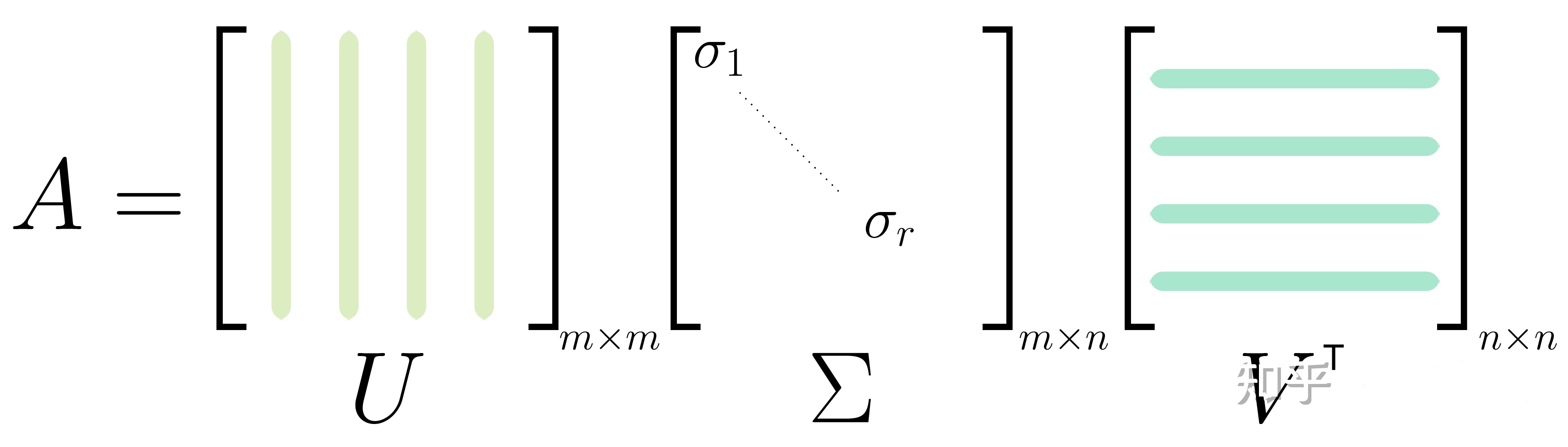
Singular Value Decomposition (SVD) is the most important decomposition method in linear algebra and has a deep connection with Principle Component Analysis (PCA) in machine learning. SVD says any matrix $A \in \mathbb{R}^{m \times n}$ of rank $r$ can be written as a product of three matrices:

where $U, V$ are orthogonal matrices. The eigenvectors of $A^{T} A$ form $V$, and the eigenvectors of $A A^{T}$ form $U$, and singular value $\sigma_ {i}=\sqrt{\lambda_ {i}\left(A^{T} A\right)}=\sqrt{\lambda_ {i}\left(A A^{T}\right)}$ is the square root of the corresponding eigenvalues. Next, we show Gilbert Strang’s derivation of $\mathrm{SVD}$[1], which is very instructive.

Derivation of SVD

• Consider an $m \times n$ matrix $A$ with rank $r$. Then $n \times n$ matrix $A^{T} A$ is symmetric and positive semidefinite since

This means the $A^{T} A$ matrix is diagonalizable with orthonormal matrix $V$ (the spectral theorem for real symmetric matrix) such that

where the eigenvalues are nonnegative $\lambda_ {i} \geq 0$ such that we can define the singular values $\sigma_ {i}=\sqrt{\lambda_ {i}}$ and order them $\sigma_ {1} \geq \sigma_ {2} \geq \ldots \sigma_ {r}>0$ .

• Notice $A^{T} A(n \times n)$ and $A(m \times n)$ have the same rank, i.e. $\operatorname{rank}\left(A^{T} A\right)=\operatorname{rank}(A)=r$, because $A \mathbf{x}=\mathbf{0}$ and $A^{T} A \mathbf{x}=\mathbf{0}$ have the same solutions, namely they have the same nullspace. First, if $\mathbf{x}$ is in the nullspace of $A$, then $A \mathbf{x}=\mathbf{0} .$ Multiplying by $A^{T}$ gives $A^{T} A \mathbf{x}=\mathbf{0} .$ So $\mathbf{x}$ is also in the nullspace of $A^{T} A$. Second, now we start with the nullspace of $A^{T} A$. From $A^{T} A=\mathbf{0}$, we multiply by $\mathbf{x}^{T}$

since for if a vector has length zero, it must be $\mathbf{0}$. We have shown that $A^{T} A$ and $A$ have the same nullspace, which means if $A^{T} A$ has dependent columns, so has $A$, and vice versa. Therefore they have the same rank.

• Let $\mathbf{v}_ {1}, \ldots, \mathbf{v}_ {r}$ be an orthonormal set of eigenvectors of $A^{T} A$ with positive eigenvalues, and orthonormal eigenvectors with zero eigenvalues, i.e. the nullspace of $A^{T} A:$

We now show that if $\mathbf{v}_ {i}$ is a unit eigenvector of $A^{T} A$ with eigenvalue $\sigma_ {i}^{2}$ then

is a unit eigenvector of $A A^{T}$ also with eigenvalue $\sigma_ {i}^{2}$.

Using orthonormal properties of basis $(\mathbf{v}_ {i})$, i.e. $\mathbf{v}_ {i}^{T} \mathbf{v}_ {j}=\delta_ {i j}$, we have

Therefore, $(\mathbf{u}_ {i}=A \mathbf{v}_ {i} / \sigma_ {i})$ are the orthonormal basis. Next, we show that $\mathbf{u}_ {i}$ is an eigenvector of $A A^{T}$ :

The $(\mathbf{u}_ {i})$ are called left singular vectors (unit eigenvector of $A A^{T}$ with eigenvalue $\left.\sigma_ {i}^{2}\right)$, and the $(\mathbf{v}_ {i})$ are called right singular vectors (unit eigenvector of $A^{T} A$ with eigenvalue $\sigma_ {i}^{2}$ ). The singular values $(\sigma_ {i})$ are the square roots of the equal eigenvalues of $A A^{T}$ and $A^{T} A$.

• If $V$ is the $n \times n$ matrix whose $i$ th column is $\mathbf{v}_ {i}, V_ {r}$ is the first $r$ columns of $V, \Sigma_ {r}$ is the $r \times r$ diagonal matrix whose $i$ th element is $\sigma_ {i}$, and $U_ {r}$ is the $m \times r$ matrix whose $i$ th column is $\mathbf{u}_ {i}=A \mathbf{v}_ {i} / \sigma_ {i}$, using orthonormal conditions $V_ {r}^{T} V_ {r}=I_ {r}$ and $U_ {r}^{T} U_ {r}=I_ {r}$, we have $A V_ {r}=U_ {r} \Sigma_ {r}:$

Multiplying both sides by $V_ {r}^{T}$ on the right, we have

• The above result is the gist of SVD, but there is more. The vectors $\mathbf{v}_ {r+1}, \ldots, \mathbf{v}_ {n}$ span the nullspace of $A^{T} A .$ But the nullspace of $A^{T} A$ is the same as the nullspace of $A$. The vectors $\mathbf{u}_ {1}, \ldots, \mathbf{u}_ {r}$ are $r$ orthonormal vectors in the column space of $A$, so they span the column space (a subspace of $\mathbb{R}^{m}$. We cam complete the set $\mathbf{u}_ {1}, \ldots, \mathbf{u}_ {r}$ with orthonormal vectors $\mathbf{u}_ {r+1}, \ldots, \mathbf{u}_ {m}$ to create full orthonormal basis of $\mathbb{R}^{m}$.

We now have $r$ triplets $\left(\sigma_ {i}, \mathbf{v}_ {i}, \mathbf{u}_ {i}\right)$, where $A \mathbf{v}_ {i}=\sigma_ {i} \mathbf{u}_ {i}$, and $n-r$ vectors $\mathbf{v}_ {r+1}, \ldots, \mathbf{v}_ {n}$ in the nullspace $N(A), m-r$ vectors $\mathbf{u}_ {r+1}, \ldots, \mathbf{u}_ {m}$ in the left nullspace $N(A^{T})$. They are automatically orthogonal to the first $r$ vectors. So if we use the complete the $V_ {n \times n}, U_ {m \times m}$ and augment diagonal matrix $\Sigma_ {m \times n}$ with zeros, we still have

Or

• Thus, we write the SVD of any matrix as below:

Orthogonal complements

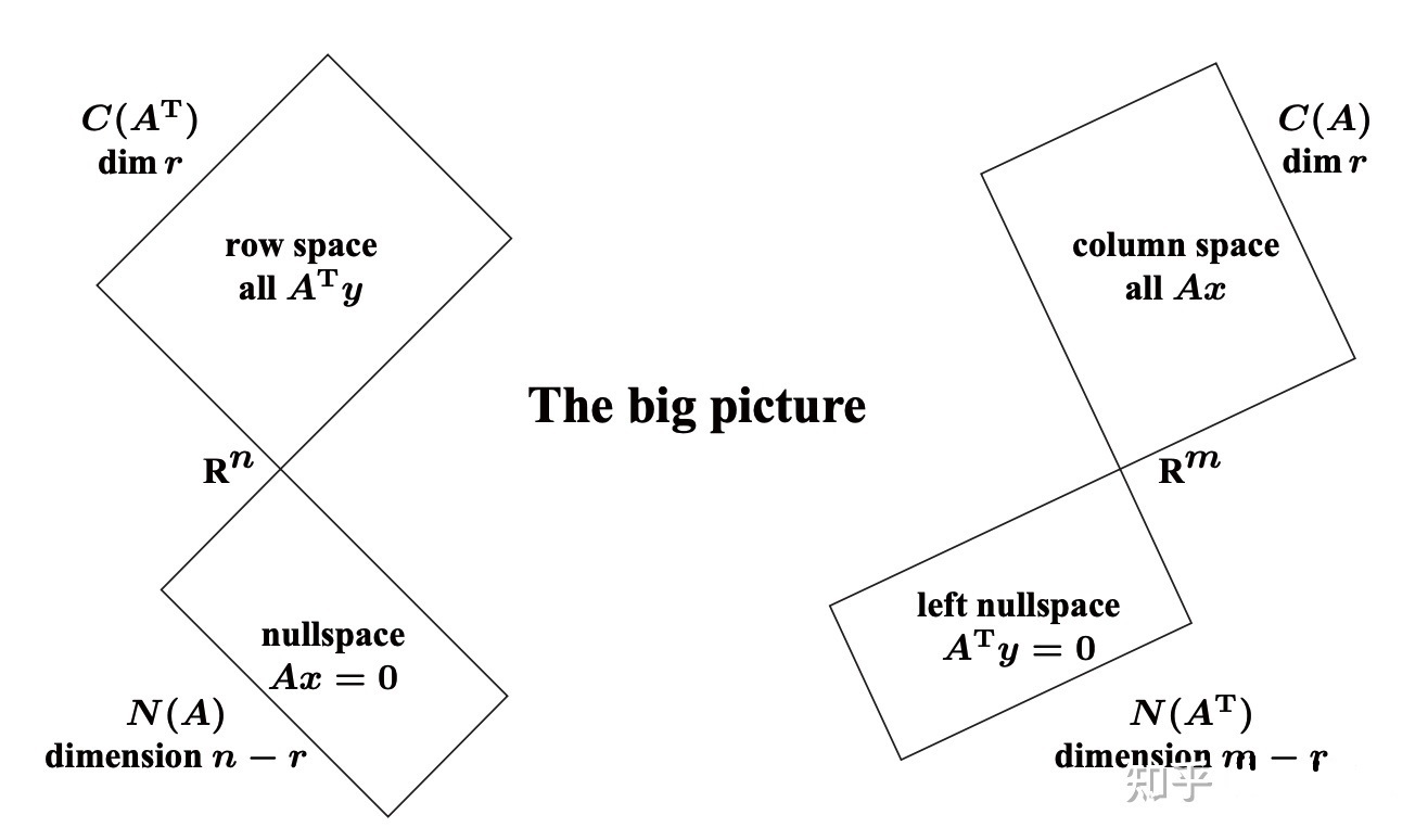
• The final beautiful comment comes from considering orthogonal complements. We have an orthonormal basis $\mathbf{u}_ {r+1}, \ldots, \mathbf{u}_ {m}$ of $\mathbb{R}^{m}$, the first $r$ of which span the column space of $A$. Therefore the remaining $m-r$ vectors $\mathbf{u}_ {r+1}, \ldots, \mathbf{u}_ {m}$ span the $C(A)^{\perp}=N\left(A^{T}\right) .$ Likewise, $\mathbf{v}_ {1}, \ldots, \mathbf{v}_ {r}$ is an orthonormal basis of $\mathbb{R}^{n}$, the last $n-r$ of which span the nullspace of $A$. Therefore the first $r$ of them span $N(A)^{\perp}=C\left(A^{T}\right)$. Thus the SVD produces not just the singular values and this nice factorization, but simultaneously a set of orthonormal bases for the four subspaces (see Fig. $3.5$ from Strang below).

The four fundamental subspaces in linear algebraSVD variants. (a) full SVD (P singular values, where P = min(M ; N )), (b) reduced/com- pact SVD (N singular values), and (c) truncated SVD (K singular values).

In summary, we have

SVD variants. (a) full SVD (P singular values, where P = min(M ; N )), (b) reduced/com- pact SVD (N singular values), and (c) truncated SVD (K singular values).

Refrences

Strang G. Introduction to linear algebra. 5th Edn Cambridge[J]. United Kingdom: Wellesley-Cambridge Press.[Google Scholar], 2016.