Abstract

In this paper, we propose a new model reduction technique aimed at real-time blood flow simulations on a given family of geometrical shapes of arterial vessels. Our approach is based on the combination of a low-dimensional shape parametrization of the computational domain and the reduced basis method to solve the associated parametrized flow equations. We propose a preliminary analysis carried on a set of arterial vessel geometries, described by means of a radial basis functions parametrization. In order to account for patient-specific arterial configurations, we reconstruct the latter by solving a suitable parameter identification problem. Real-time simulation of blood flows are thus performed on each reconstructed parametrized geometry, by means of the reduced basis method. We focus on a family of parametrized carotid artery bifurcations, by modelling blood flows using Navier-Stokes equations and measuring distributed outputs such as viscous energy dissipation or vorticity. The latter are indexes that might be correlated with the assessment of pathological risks. The approach advocated here can be applied to a broad variety of (different) flow problems related with geometry/shape variation, for instance related with shape sensitivity analysis, parametric exploration and shape design.

Introduction

In order to achieve a strong geometrical reduction and describe the carotid configurations by using only a small number of significant parameters, we introduce a general class of shape parametrizations based on the radial basis functions (RBF) technique, which is a general interpolation method based on the choice and the displacement of a small set of control points. The most original contribution in this paper is the combination of certified RB methods for viscous flows with RBF technique used to introduce a nonaffine geometrical parametrization. Given a new geometry, we may be asked to obtain a numerical approximation of the flow in a very small amount of time, say order of 1 s, that can be considered as a real-time condition.

Radial basis functions techniques for shape parametrization

Our goal is to set up a mathematical model that is flexible – in order to represent complex configurations – and low dimensional – that is depending on a small number of input parameters. Free shape representations, obtained by introducing a small set of control points – and possibly some interpolation strategies – are a good compromise between flexibility and low dimensionality, and they can be properly coupled with the RB method for parametrized PDEs. A global deformation mapping $T(\cdot ; \mu)$ is obtained as a linear combination of the control points displacements, treated as input parameters.

The RBF technique is used for nonlinear interpolation (e.g. of scattered data); in the two-dimensional $(2 \mathrm{D})$ case, a map $\tau: \mathbb{R}^{2} \rightarrow \mathbb{R}^{2}$ is defined as follows:

being $P(\cdot)$ a low-degree polynomial function; $ \left( \mathbf{w}_ {i} \right)_ {i=1}^{k} $, $ \mathbf{w}_ {i} \in \mathbb{R}^{2} $, a set of weights corresponding to the ( a priori selected) $k$ control points, whose reference positions are $\left[\mathbf{X}_ {1}, \ldots, \mathbf{X}_ {k}\right]$, a set of distinct points in $\mathbb{R}^{2} ;$ and $\sigma(\cdot)$ a (translated) radially symmetric function. Common choices introduced for modelling $2 \mathrm{D}$ (or three-dimensional (3D)) shapes are, for example

Usually, a polynomial function of degree 1 is chosen, $P(\mathbf{x})=\mathbf{c}+\mathbb{A} \mathbf{x}$, being $\mathbf{c} \in \mathbb{R}^{2}$ and $\mathbb{A} \in \mathbb{R}^{2 \times 2} ;$ thus, the map can be rewritten as

being $s(\mathbf{x})=\left(\sigma\left(\left|\mathbf{x}-\mathbf{X}_ {1}\right|\right), \ldots, \sigma\left(\left|\mathbf{x}-\mathbf{X}_ {k}\right|\right)\right)^{T} \in \mathbb{R}^{k}$ and $\mathbb{W}=\left[\mathbf{w}_ {1}, \ldots, \mathbf{w}_ {k}\right]^{T} \in \mathbb{R}^{k \times 2}$. In this way, $P(\cdot)$ is the affine part (rotation and/or scaling), whereas the term $\mathbb{W}^{T} s(\mathbf{x})$ depending on the control points adds a nonaffine contribution to the deformation. The map, Equation (17), is a function of $2 k+6$ coefficients in the $2 \mathrm{D}$ case; to compute them, we look for a transformation such that each control point of the initial (or reference) shape is mapped onto the corresponding control point of the target (or deformed) one. Introducing the initial position $\mathbb{X}=\left[\mathbf{X}_ {1}, \ldots, \mathbf{X}_ {k}\right]^{T} \in \mathbb{R}^{k \times 2}$ and the deformed position $\mathbb{Y}=\left[\mathbf{Y}_ {1}, \ldots, \mathbf{Y}_ {k}\right]^{T} \in \mathbb{R}^{k \times 2}$ of the control points, the weights $\left (\mathbf{w}_ {i}\right)_ {i=1}^{k}$ in Equation (16) are found by fulfilling the interpolation constraints

When a polynomial term $P(\mathbf{x})=\mathbf{c}+\mathbb{A} \mathbf{x}$ is included, the system is completed by the additional constraint$

being $\mathbf{X}_ {j}=\left(X_ {j 1}, X_ {j 2}\right)^{T}$, which can represent the conservation of total force and momentum [32]. Moreover, in general, if $P(\mathbf{x}) \in \mathbb{P}_ {q}=\operatorname{span}\left( p_ {1}, \ldots, p_ {Q} \right)$, space of all polynomials of degree up to $q \geq 1$ in two unknowns, the side constraints can be expressed as [19].

In order to fit the RBF technique in our parametrized framework, let us express the deformed positions $\left[\mathbf{Y}_ {1}, \ldots, \mathbf{Y}_ {k}\right]^{T}$ of the control points as

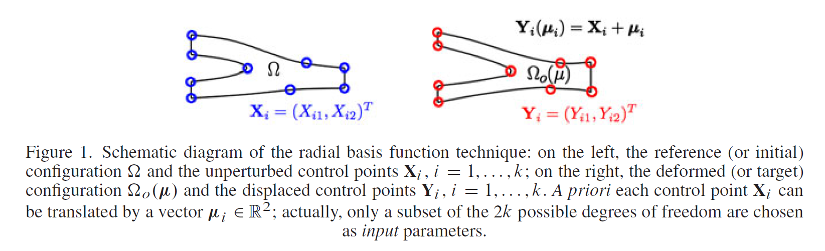
being $( \boldsymbol{\mu}_ {i}=(\mu_ {i 1}, \mu_ {i 2}))_ {i=1}^{k}$ the displacements of the $k$ control points, which are usually chosen on the boundary of the shape that has to be deformed (see Figure 1). The input parameters $\mu=\left(\mu_ {1}, \ldots, \mu_ {p}\right) \in \mathbb{R}^{p}$ are then a subset of $p \leq 2 k$ degrees of freedom, chosen accordingly to some problem-dependent criteria. Thus, the parametric mapping $T(\cdot ; \mu): \mathbb{R}^{2} \rightarrow \mathbb{R}^{2}$ will be given by

where the coefficients $c(\mu), A(\mu), \mathbb{W}(\mu)$ satisfy the constraints $(18)-(19)$. By denoting $\mathbb{S}$ the interpolation matrix whose elements are $\mathbb{S}_ {i j}=s_ {i}\left(\mathbf{X}_ {j}\right)=\sigma\left(\left|\mathbf{X}_ {j}-\mathbf{X}_ {i}\right|\right)$ and $\mathbb{I}_ {k}=[1,1, \ldots, 1]^{T} \in \mathbb{R}^{k}$, we can rewrite Equations (18) and (19) in a compact form, where the coefficients are obtained from the solution of a linear system, such that the parametrization is residing only on the right-hand side:

By adding a polynomial function $P(\mathbf{x})$ in Equation (16), the interpolation problem always admits a unique solution because the global matrix appearing in Equation (21) is symmetric and positive definite. II For a small number of control points, as in our approach, linear system (21) can be efficiently solved by a suitable direct method (matrix factorization is not depending on the parameters). When using a large number of control points $-$ as for example in fluid-structure interaction coupled problems or, more generally, when dealing with mesh motion through $\mathrm{RBF}$ - the matrix appearing in Equation (21) may be badly conditioned and non-sparse (because of the global character of RBF), and some difficulties may arise. In these cases, suitable scaling or preconditioning strategies may help, as discussed for example in [19]. Once the map $T(\cdot ; \boldsymbol{\mu})$ has been built, parametrized tensors $\boldsymbol{J}_ {T}(\boldsymbol{\mu}), \boldsymbol{v}(\boldsymbol{\mu})$ and $\chi(\boldsymbol{\mu}) \equiv \eta(\boldsymbol{\mu})$ appearing in Equation $(10)-(12)$ are computed symbolically by means of a computer algebra system.

Parameter identification for shape reconstruction

Shape reconstruction consists of recovering a transformation that establishes some desired correspondences between two geometrical configurations, according to some similarity/distance measures. In order to be compatible with the reduced real-time framework, the reconstruction procedure has to be (i) based on a small number of parameters and (ii) performed in a very small amount of time. Let us denote $\mathcal{S}$ the initial shape that has to be deformed in order to reconstruct the target shape $\mathcal{T}_ {d}$ by means of the parametric map $T(\cdot ; \mu)$. Moreover, let us introduce a shape representation $\mathcal{R}(\cdot)$, a distance (or similarity/dissimilarity metric) $d(\cdot)$ defined in the space of representations and a loss function $\rho(\cdot)$. The reconstruction process can be, in general, expressed as a minimization problem:

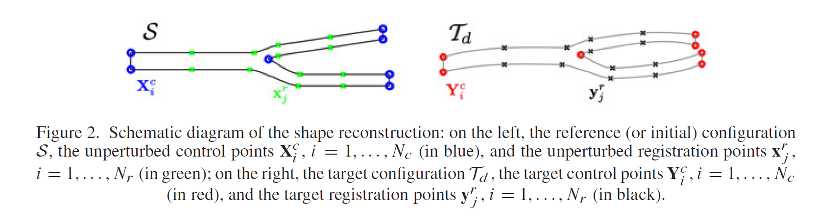
where $\mathcal{D}_ {a d}$ is the space of admissible parameters, $\omega(\boldsymbol{\mu})$ is a suitable regularization term and $\beta>0$ is a weighting parameter. A usual choice is $\rho(s)=s^{2}$ for the loss function and the Euclidean distance for $d(\mathbf{x})$; more complex transformations or weighting can be introduced in order to improve the robustness of the matching. The most difficult task is the choice of the shape representation $\mathcal{R}(\cdot)$. Many strategies have been developed [33, 34]. In view of model reduction, we represent a shape configuration by means of a set of $N_ {r}$ registration points (or landmarks) $(\mathbf{x}_ {j}^{r})_ {j=1}^{N_ {r}} \in \mathcal{S}$, such that $\mathcal{R}(T(\mathcal{S} ; \boldsymbol{\mu}))=T(\mathbf{x}_ {j}^{r} ; \boldsymbol{\mu}), \quad r=1, \ldots N_ {r}$; in the same way, we suppose to know the target position $\mathcal{R} (\mathcal{T}_ {d})=(\mathbf{y}_ {j}^{r})_ {j=1}^{N_ {r}}$ of these registration points in the target configuration $\mathcal{T}_ {d}$. Moreover, we introduce a set of control points $\left(\mathbf{X}_ {i} \right)_ {i=1}^{N_ {C}}$ on the initial shape in order to define a parametric RBF mapping $T(\cdot ; \mu)$, whose image is given by $\left( \mathbf{Y}_ {i}\right)_ {i=1}^{N_ {C}}$ (see Figure 2 for a summarizing scheme). The idea is that, because the RBF mapping may fail in matching the two configurations, the registration points can be used to drive the mapping in order to enhance its fitting capabilities. In this way, the parameter identification problem (22) becomes a matching problem between two point-sets, which can be written as a least squares minimization problem

where the regularization term (a quadratic function of $\mu$ ) is given by the distance between the images $\left( T (\mathbf{X}_ {i}^{c} ; \mu) \right)$ of the control points and their target positions $( \mathbf{Y}_ {i})_ {i=1}^{N_ {C}}$. Note that the introduction of the registration points does not increase the problem dimension, as the number of input parameters of shape representation remains unchanged. Concerning the control points, they need to be scattered all over the domain in order to describe a wide family of shapes and global deformations.

References

Manzoni A, Quarteroni A, Rozza G. Model reduction techniques for fast blood flow simulation in parametrized geometries[J]. International journal for numerical methods in biomedical engineering, 2012, 28(6-7): 604-625.