1.Parametrized partial differential equations
| notation | meaning |
|---|---|
| $\Omega$ | $\Omega \subset \mathbb{R}^{2}$, a fixed, parameter-independent domain |
| $\widetilde{\Omega}$ | $\widetilde{\Omega}=\widetilde{\Omega}\left(\boldsymbol{\mu}_ {g}\right) \subset \mathbb{R}^{2}$, the computational domain |
| $\boldsymbol{\mu}_ {p h}$ | $\boldsymbol{\mu}_ {p h} \in \mathscr{P}_ {p h}$, physical parameters, addresses material properties, source terms and boundary conditions |
| $\boldsymbol{\mu}_ {g}$ | $\boldsymbol{\mu}_ {g} \in \mathscr{P}_ {g}$, geometrical parameter, defines the shape of the computational domain |
| $\boldsymbol{\mu}$ | $\boldsymbol{\mu}=\left(\boldsymbol{\mu}_ {p h}, \boldsymbol{\mu}_ {g}\right) \in \mathscr{P}=\mathscr{P}_ {p h} \times \mathscr{P}_ {g} \subset \mathbb{R}^{P}$, the overall input vector parameter |
| $\widetilde{\Gamma}_ {D}\left(\boldsymbol{\mu}_ {g}\right)$ | Dirichlet boundary conditions of $\widetilde{\Omega}\left(\boldsymbol{\mu}_ {g}\right)$ |
| $\widetilde{\Gamma}_ {N}\left(\boldsymbol{\mu}_ {g}\right)$ | Neumann boundary conditions of $\widetilde{\Omega}\left(\boldsymbol{\mu}_ {g}\right)$ |
| $\widetilde{V}$ | a Hilbert space $\widetilde{V}=\widetilde{V}\left(\boldsymbol{\mu}_ {g}\right)=\widetilde{V}\left(\widetilde{\Omega}\left(\boldsymbol{\mu}_ {g}\right)\right)$ defined over the domain $\widetilde{\Omega}\left(\boldsymbol{\mu}_ {g}\right)$ |
| $\widetilde{V}^{\prime}$ | the dual space of $\tilde{V}$ |
| $\widetilde{G}$ | $\widetilde{G}: \widetilde{V} \times \mathscr{P}_ {p h} \rightarrow \widetilde{V}^{\prime}$ the map representing a parametrized nonlinear second-order PDE |
| $\Phi$ | $\Phi: \Omega \times \mathscr{P}_ {g} \rightarrow \Omega$ the parametrized map |
The differential (strong) form of the problem of interest reads: given $\boldsymbol{\mu}=\left(\boldsymbol{\mu}_ {p h}, \boldsymbol{\mu}_ {g}\right) \in \mathscr{P}$, find $\widetilde{u}(\boldsymbol{\mu}) \in \widetilde{V}\left(\boldsymbol{\mu}_ {g}\right)$ such that
\[\widetilde{G}\left(\widetilde{u}(\boldsymbol{\mu}) ; \boldsymbol{\mu}_ {p h}\right)=0 \quad \text { in } \tilde{V}^{\prime}\left(\boldsymbol{\mu}_ {g}\right). \tag{1} \label{eq1}\]namely
\[\left\langle\widetilde{G}\left(\widetilde{u}(\boldsymbol{\mu}) ; \boldsymbol{\mu}_ {p h}\right), v\right\rangle_ {\tilde{V}^{\prime}, \tilde{V}}=0 \quad \forall v \in \widetilde{V}\left(\boldsymbol{\mu}_ {g}\right)\]with $\langle\cdot, \cdot\rangle_ {\tilde{V}^{\prime}, \tilde{V}}: \widetilde{V}^{\prime} \times \widetilde{V} \rightarrow \mathbb{R}$ the duality pairing between $\widetilde{V}^{\prime}$ and $\tilde{V}$. The finite element method requires problem $\eqref{eq1}$ to be stated in a weak (or variational) form . To this end, let us introduce the form $\widetilde{g}: \widetilde{V} \times \widetilde{V} \times \mathscr{P} \rightarrow \mathbb{R}$, with $\widetilde{g}(\cdot, \cdot ; \boldsymbol{\mu})$ defined as:
\[\widetilde{g}(w, v ; \boldsymbol{\mu})=\left\langle\widetilde{G}\left(w ; \boldsymbol{\mu}_ {p h}\right), v\right\rangle_ {\tilde{V}^{\prime}, \tilde{V}} \quad \forall w, v \in \widetilde{V}\]The variational formulation of $\eqref{eq1}$ then reads: given $\boldsymbol{\mu}=\left(\boldsymbol{\mu}_ {p h}, \boldsymbol{\mu}_ {g}\right) \in \mathscr{P}$, find $\widetilde{u}(\boldsymbol{\mu}) \in \widetilde{V}\left(\boldsymbol{\mu}_ {g}\right)$ such that
\[\widetilde{g}(\widetilde{u}(\boldsymbol{\mu}), v ; \boldsymbol{\mu})=0 \quad \forall v \in \widetilde{V}\left(\boldsymbol{\mu}_ {g}\right)\]2.From physical to reference domain
When addressing problems defined on variable shape domains, ensuring the compatibility among snapshots is crucial. To this end, it is practice to formulate and solve the differential problem over a fixed, parameter-independent domain $\Omega \subset \mathbb{R}^{2}$. This can be accomplished by introducing a parametrized map $\Phi: \Omega \times \mathscr{P}_ {g} \rightarrow \Omega$ such that fixed and parameter-independent domain
\[\widetilde{\Omega}\left(\boldsymbol{\mu}_ {g}\right)=\mathbf{\Phi}\left(\Omega ; \boldsymbol{\mu}_ {g}\right)\]The transformation $\mathbf{\Phi}\left(\cdot ; \boldsymbol{\mu}_ {g}\right)$ allows one to restate the general problem $\eqref{eq1}$. Let $V$ be a suitable Hilbert space over $\Omega$ and $V^{\prime}$ be its dual. Suppose $V$ is equipped with the scalar product $(\cdot, \cdot)_ {V}$ and the induced norm $|\cdot|_ {V}=\sqrt{(\cdot, \cdot)_ {V}}$. Given the parametrized map $G: V \times \mathscr{P} \rightarrow V^{\prime}$ representing the (nonlinear) PDE over the reference domain $\Omega$, we focus on problems of the form: given $\boldsymbol{\mu} \in \mathscr{P}$, find $u(\boldsymbol{\mu}) \in V$ such that 1Omiga : reference domain
\[G(u(\boldsymbol{\mu}) ; \boldsymbol{\mu})=0 \quad \text { in } V^{\prime} \tag{2} \label{eq2}\]The weak formulation of problem $\eqref{eq2}$ reads: given $\boldsymbol{\mu} \in \mathscr{P}$, seek $u(\boldsymbol{\mu}) \in V$ such that
\[g(u(\boldsymbol{\mu}), v ; \boldsymbol{\mu})=0 \quad \forall v \in V\]where $g: V \times V \times \mathscr{P} \rightarrow \mathbb{R}$ is defined as
\[g(w, v ; \boldsymbol{\mu})=\langle G(w ; \boldsymbol{\mu}), v\rangle_ {V^{\prime}, V} \quad \forall w, v \in V, \forall \boldsymbol{\mu} \in \mathscr{P}\]with $\langle\cdot, \cdot\rangle_ {V^{\prime}, V}: V^{\prime} \times V \rightarrow \mathbb{R}$ the dual pairing between $V$ and $V^{\prime}$. Observe that the explicit expression of $g(\cdot, \cdot ; \boldsymbol{\mu})$ involves the $\operatorname{map} \mathbf{\Phi}\left(\cdot ; \boldsymbol{\mu}_ {g}\right)$, thus keeping track of the original domain $\widetilde{\Omega}\left(\boldsymbol{\mu}_ {g}\right)$. Then, the solution $\widetilde{u}(\boldsymbol{\mu})$ over the original domain $\widetilde{\Omega}\left(\boldsymbol{\mu}_ {g}\right)$ can be recovered as
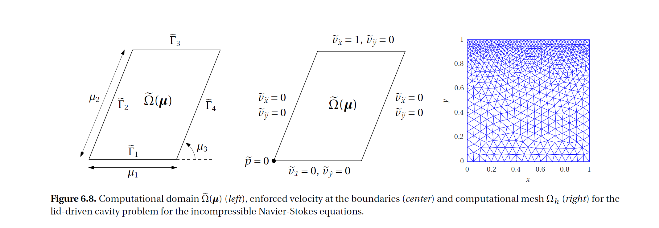
\[\tilde{u}(\boldsymbol{\mu})=u(\boldsymbol{\mu}) \circ \boldsymbol{\Phi}\left(\boldsymbol{\mu}_ {g}\right)\]In our numerical tests, we employ the squared reference domain shown on the right in Fig. $6.3$ and we resort to a particular choice for $\mathbf{\Phi}\left(\cdot ; \boldsymbol{\mu}_ {g}\right)$ - the boundary displacement-dependent transfinite map (BDD TM).
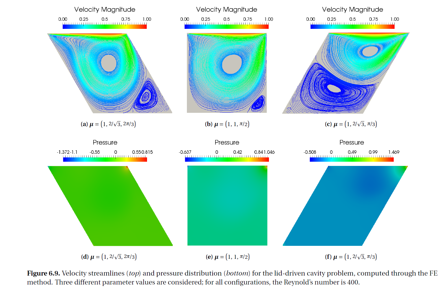
3.Numerical results